Goals

• Understand how the binomial distribution can be applied to scientific questions
• Learn how to calculate the binomial distribution using R
• Learn how to do a binomial test using R, including practicing the steps in hypothesis testing

Review the quick summary of the chapter on Canvas, and you may want to look at the steps in hypothesis testing handout on Canvas.

Introduction

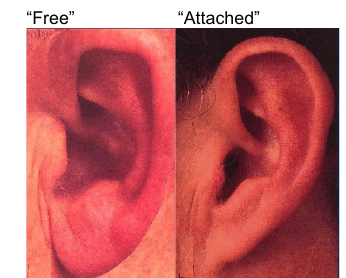
Nearly all biological populations are genetically variable. Today we will focus on a genetically variable morphological trait that is easy to score: whether a person’s ear lobe is “free” or “attached” (see below). The typical frequency of the “free” phenotype is 0.65, although there is variation around the world.

Step 2: Recall that the probability of obtaining X successes and is defined as: where .

We will arbitrarily define a “success” as a person with a “free” ear lobe. Imagine you want to know: Given that the probability of a “free” ear lobe is 0.65, what is the probability of collecting your sample (i.e. X people with a “free” ear lobe in a group of n = _______ people?)

Question 1. What is this probability? To answer this question, state the numerical value of n, p, and X, write out the appropriate binomial formula for this problem, and then solve the formula.

Now ^[a] check your calculations for Question 1 using RStudio. You can do this by setting x, n, and p variables to correspond to the values that you are interested in.

Did you get the same answer as you calculated by hand?

Step 3: The binomial test is a form of the hypothesis testing we did in Chapter 6. We will address the following question:

“In a randomly selected group of n=20 students, there were x=8 students with free earlobes. Is this result consistent with a population with 65% free ear lobes?”

Question 2: Write down the appropriate null and alternative hypotheses. State these hypotheses both with words and with symbols (i.e. stating the value of p).

Step 4: We will treat our sample as random. The next step in hypothesis testing is to calculate some descriptive statistics, including our test statistic. For the binomial test, the test statistic is simply the number of successes. Next we need to determine how compatible the data are with the null hypothesis (i.e. calculate theP-value). To do this we need to calculate the null distribution. The null distribution is the sampling distribution of outcomes for the test statistic under the assumption that the null hypothesis is true.

The binomial distribution is the null distribution for the binomial test. We will use R to calculate the null distribution. Recall that a probability distribution assigns a probability about every possible value for a variate. If you have n=20 in your lab section, then the domain of possible X values is 0, 1, 2, … , 20. In R you can create a vector with this range easily (after you assign the correct value to n) using the : syntax:

p = 0.65
x = put the # of people with "free" in example
n = total number of in example
domain = 0:n

Because R happily operates on a vector of arguments rather than just one argument, we can find the probability of every possible X value using the same dbinom function we used above:

null.dist = dbinom(domain, n, p)
print(paste(c("The null distribution is: ", null.dist)))

Step 5: Of course it is more pleasant to look at a graph of the null rather than a vector of probabilities. Execute the following:

barplot(null.dist, names.arg=domain)

(a histogram would be more appropriate than a barplot, but it is trickier to generate - we will just ignore the spaces between the bars for the sake of this lab).

Question 4a:

You can check this withsum(null.dist)

Question 4b: Look at the graph: State what the x axis and y axis should be labeled.

Question 4c: What is the “expected” number of individuals with “free” ear lobes given the null hypothesis (= expected number of successes)?

To answer 4c read the graph, but also execute the following:

expected = n*p
print(paste(c("The expected value under the null is: ", expected)))

The product np is the mean of the binomial distribution. Can you see why it makes sense that this product would tell you the expected number of successes if the null hypothesis was true?

Step 6:  Now let’s figure out how to answer:

Question 4d:  What is the probability of getting the observed data ( x  individuals with free lobes) or more extreme data, assuming the null hypothesis is true?

First we will figure out how far our real data deviated from the expectation under the null:

obs.diff = x - expected

print(paste("The difference between the observed and the expected was", obs.diff))

So, now we can figure out which possible values in full domain of X  are “more extreme” than our real data. Because we would be surprised by values that are larger or smaller than the expected value, we should use the abs  function to look at the absolute value of the differences between the X  and the expected:

as.extreme = abs(domain - expected) >= abs(obs.diff)

print("The tails of the distribution will correspond to TRUE values:")

print(as.extreme)

Now the vector as.extreme should identify which elements are in the tails of the distribution.

We can make our barplot color in the tails with a bit of arcane syntax. This sets up a color vector of white and red, then we rely on a trick that the numeric interpretation of TRUE in R is 1. This lets us create a vector for each element in our domain with red for the values in the tail of the distribution.

col = c("white", "red")

x.col = col[1 + as.numeric(as.extreme)]

barplot(null.dist, names.arg=domain, col=x.col)

The plot is nice, but question 4d asked for the probability. Since we are considering a complex event best thought as “The probability of X=0 OR X=1 OR…”  we can use the addition rule.

prob.as.extreme = sum(null.dist[as.extreme])

z = paste("If the null is true, the prob. of a stat at least as extreme as",             x, "is", prob.as.extreme)

Step 7: Question 4e:  What is the P-value for this test?

Step 8: Make a decision regarding the null hypothesis, assuming that alpha = 0.05.

Question 5 . State whether you reject or “do not reject” the null hypothesis.

Step 9: Conclude by answering the original question and reporting the results of the study. Question 6 . In complete and logical sentences, provide the results of the study. One typically reports the descriptive statistics, sample size, test statistic, and P -value as part of this summary. However, in this case, your descriptive statistics and test statistic are the same value, so you don’t have to restate them twice.

Remember: if you reject the null hypothesis, it is appropriate (and important!) to state the “directionality” of the data. That is, if you reject the null hypothesis, you are not only concluding that your data suggests that the population proportion is not equal to p0  but you additionally know the direction of deviation.

For example, for this problem, if you reject the null hypothesis, you can state that the population your sample was taken from has either a higher or lower proportion of free ear lobes than is stated in the null hypothesis.

Note: In the above procedure, we calculated an “exact” P -value. You may note that your book (p. 187–188) takes a “shortcut” and approximates the P -value by calculating two times the area of one “tail”. We are adding up each tail to clearly show the meaning of the P-value.

Step 10:  There are easier ways to calculate the P - value of binomial test in R. In this example, the tails of the distribution were delimited by 8 and 18 (including those endpoints). The pbinom(x, n, p)  function returns the cumulative probability associated with the having any . So, we can get the P -value using the following shortcuts to calculating probabilities using binomial distribution:

print(paste("Pr(x <= 8) =", pbinom(8, n, p)))

print(paste("Pr(x <= 17) =", pbinom(17, n, p)))

print(paste("Pr(x > 17) =", 1 - pbinom(17, n, p)))

print(paste("Pr(in tails) =", pbinom(8, n, p) + 1 - pbinom(17, n, p)))

Optional Step 11:  Below are some more examples of the binomial test for you to practice with on R. We strongly encourage you to work through as many of these as you can during this laboratory session, when you can ask your TA for help.

We use a binomial test when we have a categorical response variable with 2 outcomes (“free” vs . “attached” in the earlobe example) and the null hypothesis is that each trial has the some specific probability of a “success” ( p 0  = 0.65 in our example).

As with all tests that we cover in this course, the test works by quantifying whether the sample data are consistent with the null. If so, we should “not reject the null hypothesis”. Alternatively, if there is a very low probability of collecting our particular sample data from a population with proportion p 0 , we should “reject the null hypothesis”.

Ask your TA if you are uncertain about how to apply the binomial test to each of these problems. For each problem below, state the null and alternative hypotheses (assume two-tailed hypotheses), determine your test statistic, calculate the null distribution and P-value, and state your results. Assume that the data presented are a random sample.

To use R to calculate your P-value, for each example below identify p, x, and n and use the following code to print out the probability distribution. You can then identify the probabilities that need to be summed and use them to calculate your P-value or if you are comforatble you can edit the shortcuts above do this for you in one line of code.

Example 1) Based on vital statistics, 20% of the deaths for individuals who are 55-64 years old are due to cancer. In a group of 55-64 year olds that work in a nuclear-power plant, 4 of 10 individuals have cancer. Do these data suggest that incidence of cancer in nuclear power workers is different from the general population?

Example 2) As our planet warms, the temperature change will affect species distributions. A recent study of the range limits of European butterflies found that, of 24 species that had changed their ranges in the last 100 years, 22 of them had moved farther north and only two had moved further south. Determine whether there is evidence that the fraction of butterfly species that moves north is different from the fraction that moves south.

Example 3) A scientific paper states that 90 percent of men can perceive all colors; the rest are red/green colorblind. The latter causes problems with traffic signals. 30 men are randomly chosen for a study of traffic signal perceptions. A researcher summarized the sample data and stated that 83.3 percent of the men could perceive all colors. Do these data suggest an incidence of vision types in this population that is different from that reported in the literature?

Example 4) After being rejected for employment at the Smith Corporation, Sue learns that the company has hired six women among the last 20 new employees. She also learns that the pool of applicants is large, with an approximately equal number of qualified men and women. Is there evidence to support Sue’s concern of gender-discrimination?